Past, Present, and Forecasts: Time Series Visualization with Style

Add clarity to Plotly charts by combining line styles, annotations, and background shading.

Apr 08, 2025

I’ve been reading Cole Nussbaumer Knaflic’s book Storytelling with Data (see Notes) - it’s quite illuminating. However, the author does not attempt to provide any implementation details, so I’m trying to remedy that.

When working with time series data, we often blend the certainty of historical records with the uncertainty of future projections. This is particularly true when dealing with financial data, where you tell a story of how current events might influence future trends. But if current and future data are rendered similarly in a chart, your audience might miss the difference or misinterpret your insights.

In this article, we’ll use Python and Plotly to visualize a time series where the past and future are clearly distinguished using thoughtful design choices. Whether you’re presenting forecasts, planning reports, or just want cleaner charts, this guide will help you level up your data storytelling.

Why Visual Distinction Matters

When visualizing time series data, it’s easy to fall into the trap of treating all data equally. But there’s clearly a huge difference between what has already happened and what we expect to happen. If we don’t make that distinction visually clear, we might risk confusing the audience.

Say we’re presenting a forecast of sales growth. If our projected values are rendered with the same styling as historical data, are we implying that the future is just as certain as the past?

Visual design is our opportunity to signal uncertainty. A dashed line can indicate something is estimated. A shaded background might subtly cue that we’re entering a new phase. An annotation helps clarify meaning right on the chart, reducing the need for footnotes or explanations in your text.

Good design doesn’t just make better-looking charts — it makes them more honest and more effective.

Setting Up Your Data

We’ll start with some fictional data and build a chart step by step. We will use Plotly Graphic Objects, as this library is straightforward to use and gives us more flexibility than Plotly Express.

I’ll present the code as cells from a Jupyter Notebook (the code will be available in my GitHub repo shortly after publication — see the link at the end of the article). If you prefer a plain old Python program, then just concatenate the code cells and it should work fine.

Before we define the data, we should import the libraries.

import plotly.graph_objects as go
import pandas as pd

import plotly.io as pio
pio.templates.default = "plotly_white"

Now, I must admit to having a thing about the default Plotly theme: I don’t much like it, so I almost always set the default theme to ‘plotly_white’, which I find to have a much cleaner look. Also, for this exercise, we want the plain white background that this theme gives us. The last two lines of code ensure that this theme is used throughout.

The data is just a set of integers and dates. We can imagine that they are sales figures of some sort, although this is not important. The important thing is that they are split into historical figures and projected ones. The data covers 15 years from 2015 to 2029, and I’m assuming that you are reading this in 2025, so the first 9 years are historical data and the final 6 years are predicted values.

# Sample data
data = {
    "Date": pd.date_range(start="2015-01-01", periods=15, freq="YE"),
    "Value": [10, 15, 20, 25, 30, 20, 35, 40, 38, 45, 50, 55, 60, 62, 65],
}

df = pd.DataFrame(data)

# Split into historical and projected data
historical = df.iloc[:10]  # First 10 years
projection = df.iloc[9:]   # Last 6 years

The sample data is created as a range of 15 datetimes with a frequency of 1 year and a list of 15 integer values. We create a data frame from this and then split the original dataframe into the first 10 and last 5 years. The result is two dataframes historical and projection which contain the historical data and the predicted data, respectively.

3. Plotting with Plotly Graphic Objects

To create a chart with Plotly Graphic Objects (GO), we first create a GO object and then add traces (i.e. plots).

To plot a line chart, we use the method go.scatter() to produce a trace and add that to the figure. That’s right, a scatter plot. But we set the mode parameter to ‘lines’, which tells the method to use lines instead of dots as the marker for plotting — a scatter plot that uses lines to plot each point is, of course, a line plot.

The code to plot the historical data is shown below where you can see that we set the x and y parameters to the Date and Value fields of the dataframe and specified the line colour to be blue.

# Create the figure
fig = go.Figure()

# Add historical data
fig.add_trace(go.Scatter(
    x=historical["Date"], 
    y=historical["Value"], 
    mode="lines", 
    name="Historical",
    line=dict(color="blue")
))

fig.show()

The resulting plot is shown below.

That is the first 10 years of data.

Now let’s add in the projected data.

# Add projected data with a dashed line
fig.add_trace(go.Scatter(
    x=projection["Date"], y=projection["Value"], mode="lines", name="Projection",
    line=dict(color="blue", dash="dash")
))

fig.show()

This is pretty similar to the previous code, but it uses the second dataframe and sets the line style to be dashed. Adding this trace creates a new plot that builds on the old one.

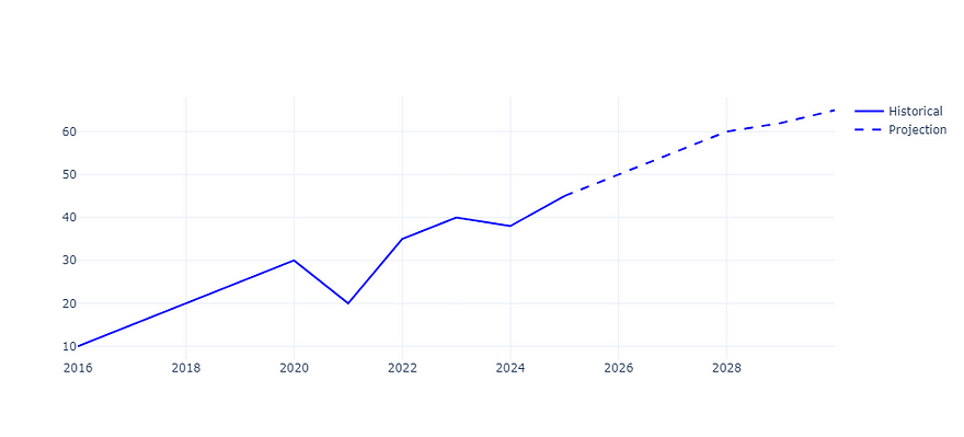
Plotly GO has automatically added a legend so that we can see what the different traces mean. However, even without that textual clue, it is very clear from the visual look of the plots that the data are different.

Enhancing with Graph Objects

It is hard to envisage a graph that does not need some sort of textual description to set the context. So, let’s add some basic text: a title and labels for the axes.

# Update layout
fig.update_layout(
    title="Historical Sales Data and Projected Sales",
    xaxis_title="Year",
    yaxis_title="Units Sold",
    xaxis=dict(showgrid=False),
    yaxis=dict(showgrid=True),
    showlegend=False
)

# Show plot
fig.show()

The update_layout method does exactly what it says, it allows us to change aspects of the plot. Here we have added the text fields as mentioned and set the grid to horizontal lines only. We also removed the legend.

Here’s the new version.

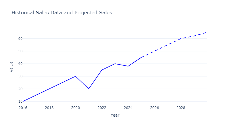
That is looking good, already, but we are going to further distinguish between the two types of data.

The following code cell adds a shaded area to the projected data.

# Add a shaded background for the projection period
fig.add_shape(
    type="rect",
    x0=projection["Date"].iloc[0], x1=projection["Date"].iloc[-1],
    y0=0, y1=1,  # Covers full y-axis
    xref="x", yref="paper",
    fillcolor="lightblue", opacity=0.3, layer="below"
)
fig.show()

Next, we add a textual annotation to describe that area.

# Add annotation for projection period
fig.add_annotation(
    x=projection["Date"].iloc[2],  # Middle of the projection period
    y=max(df["Value"]) * 1.1,  # Slightly above max value
    text="Projected data",
    showarrow=False,
)
fig.show()

The chart now looks like this.

The projections are now easily distinguished as they are contained in that shaded box.

For consistency, I have written code to similarly contain the historical data. Frankly, I’m not sure that this is absolutely necessary, but here it is anyway.

# Add a shaded background for the historical period
fig.add_shape(
    type="rect",
    x0=historical["Date"].iloc[0], x1=historical["Date"].iloc[-1],
    y0=0, y1=1,  # Covers full y-axis
    xref="x", yref="paper",
    fillcolor="lightgrey", opacity=0.3, 
    layer="below"
)

# Add annotation for historical period
fig.add_annotation(
    x=historical["Date"].iloc[2],  # Middle of the projection period
    y=max(df["Value"]) * 1.1,  # Slightly above max value
    text="Historical Data",
    showarrow=False,
)

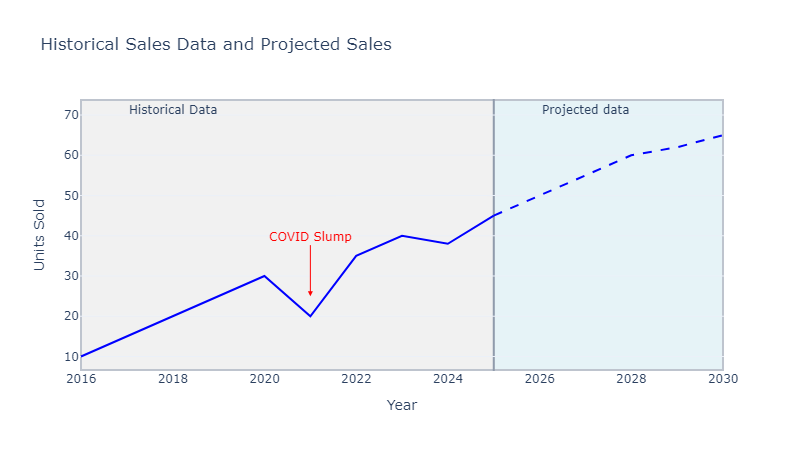
fig.show()

This treats the historical data in the same way as the projections but the shading is a different colour.

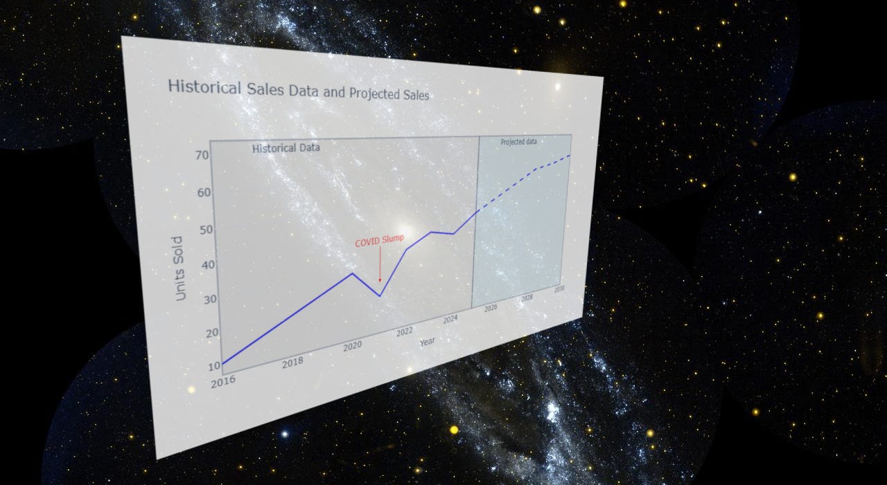
The resulting chart clearly shows the purpose of each section of the data and so the chart does not require a legend.

Annotating specific events

If you had been hiding under a rock for the last few years, or have a very short memory, then you might be confused by the slump in sales in the middle of the historical period. To allay the fears of sales executives who are not paying attention, we can add text to the graphs to explain such anomalies.

Plotly GO allows us to add text, as we saw above, but we can also add nice little arrows to highlight a point in the graph.

# Add annotation for COVID in 2020
fig.add_annotation(
    x=pd.Timestamp("2020-12-31"),  # Year 2020
    y=25,  # Position above the value for 2020
    text="COVID Slump",
    showarrow=True,
    arrowhead=2,
    arrowsize=1,
    arrowcolor="red",
    ax=0, ay=-60,  # Arrow pointing down
    font=dict(size=12, color="red")
)
# Show plot
fig.show()

The code above positions a text annotation and defines an arrow that points to a particular part in the graph.

That is my final version of the graph.

Final Thoughts

We’ve demonstrated how Plotly Graphic Objects can be used to create clear and easy-to-interpret graphs.

Different line styles help distinguish between various data types, and grouping them within shaded boxes further enhances clarity.

Textual annotations and labels are crucial for providing context and can also be used to draw attention to specific areas of interest.

Data visualization is fundamentally about communication, and I hope the examples shown highlight how well-designed, visually appealing charts can enhance that communication.

While the data used here is simple and fictional, the techniques are applicable to your own real-world datasets.

Share Hands on Data Visualization, Data Science, AI and Python

As ever, thanks for reading and I hope that this has been useful. To see more of my articles, follow me on Medium or subscribe to my Substack.

The code and data for this article can be found in my GitHub repo. I will place a link to it here shortly after publication.

Notes

I have been very much influenced by Cole Nussbaumer Knaflic’s book Storytelling with Data: A Data Visualization Guide for Business Professionals. It’s well worth a read if data visualisation is your thing. It’s available here (affiliate link).
I messed up the presentation of the date of the Covid pandemic, but I’d already created all the code and images and practically finished the article before I noticed. And I’m too darned lazy to do it over. Sorry!

Currently, although paid subscriptions are open, you won’t get anything extra - this may change in the future. But if you feel inclined to support my work regularly, you could do this. If you don’t want to, that’s fine, just take out a free subscription. Or, if you don’t want to get stuff in your inbox, just follow me.

Or…

Hands on Data Visualization, Data Science, AI and Python